Blog Post Six: The Ground Game
October 19, 2022
Introduction
In this blog post, I will think carefully about how to incorporate voter turnout into my model, and combine this analysis with my existing findings about the economy, incumbency, and expert predictions. I will also move from a linear model to a generalized linear model, forecasting a binomial vote distribution for each district instead of a single point estimate of Democrat vote share.
Thinking About Turnout
As we saw last week, the “air war” did not impact our predictive model very much, because the coefficient on our advertisement spending data was very low. Our interpretation of this was that it fell in line with findings from by Gerber et al. that advertisements have have an effect that deteriorates almost completely after one week.
We know, thanks to Huber and Arceneaux, that campaign advertisements do not generally mobilize voters to go to the polls when they otherwise would have stayed home; rather, they subliminally persuade voters to change how they approach the decision of who to vote for. However, we also know, thanks to Enos and Fowler, that the “ground game” legitimately does mobilize voters to get to the polls when they otherwise would not have. The composition of the voter pool likely impacts the result of an election, so we would like to incorporate this information into our predictive models. Unfortunately, we do not have access to detailed data about ground game operations on the district level, like the number of field offices or campaign employees. What we do have access to is somewhat robust data on advertising spending, which we know correlates with ground game activities.
So, I propose using campaign advertising spending as a proxy for ground game activity, with which we can predict voter turnout. We want to predict voter turnout as a first step since our ultimate goal is to forecast the 2022 midterm elections, and we of course do not know what voter turnout will look like on November 8th!
Below presents a simple regression model predicting the voter turnout (as a percentage of the civilian voting age population of the district) from the total campaign advertisement spending in the district (from all parties), and from the voter turnout in the previous election. In this case, by “previous election” I mean the election from four years ago, so that midterm elections line up and presidential elections line up. This is because voter turnout is much higher in presidential years, due to the high stakes office being elected. Also, the campaign spending data gives us information like the tone and purpose of each ad, which might give us a clue about the style of the ground game used in this district, but Kalla and Broockman find that the ground game does not persuade voters very effectively. So the tone/purpose of the campaign in each district is not relevant for our purposes - we only need to focus on the volume of the campaign. We use the total spending in each district over the entire campaign, not a transformation of it (e.g. its logarithm), because Enos and Fowler demonstrate that ground game efforts are approximately additive (contrasting with Gerber et al.’s finding that the air war is not).
##
## Call:
## lm(formula = Turnout ~ TotalSpending + TurnoutPrev, data = df1)
##
## Residuals:
##      Min       1Q   Median       3Q      Max
## -27.8602  -3.0798   0.1149   2.8729  13.3524
##
## Coefficients:
##                Estimate Std. Error t value Pr(>|t|)
## (Intercept)   3.068e+01  1.145e+00  26.801  < 2e-16 ***
## TotalSpending 5.776e-07  8.541e-08   6.763 6.48e-11 ***
## TurnoutPrev   4.937e-01  2.558e-02  19.295  < 2e-16 ***
## ---
## Signif. codes:  0 '***' 0.001 '**' 0.01 '*' 0.05 '.' 0.1 ' ' 1
##
## Residual standard error: 5.318 on 319 degrees of freedom
##   (408 observations deleted due to missingness)
## Multiple R-squared:  0.5749, Adjusted R-squared:  0.5722
## F-statistic: 215.7 on 2 and 319 DF,  p-value: < 2.2e-16
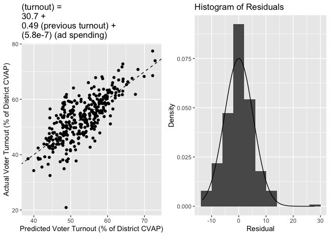
This model explains 57.5% of the variance in voter turnout, which is fairly good - the scatterplot comparing predicted voter turnout with actual voter turnout is pretty closely aligned with the dashed 45-degree line. Moreover, our coefficient for advertisement spending is statistically significant, and is large enough that it will affect our model. Even though a coefficient on the order of 10−7 might seem small, the mean advertisement spending in the data is roughly 2 × 10⁷, quite large. According to our model, this level of campaign spending would cause roughly a 1.2% increase in voter turnout in the district, which is on the same order of magnitude of estimates of the effect of the ground game that we see in the literature. This validates our simple model.
Not only is predicting turnout important because we do not know what the 2022 turnout will look like, but our model gives us the voter turnout that is implied by the ground game in the district. This is an interpretation that we care about, since it allows us to measure the campaign’s effect on the election (instead of the effect of some voters waking up on Election Day and randomly deciding to go vote). So, in training our generalized linear model, we will actually use this estimate for voter turnout instead of the actual voter turnout, because it allows us to learn about the effectiveness (or, lack thereof) of campaigns.
Model Update
Now, we will move on to updating our main predictive model for 2022. The major update is moving from a linear model that predicts Democrat vote share to a generalized linear model that predicts the probability of the Democrat candidate’s success. The specific GLM we will use is a binomial logistic model, where we assume that each voter casts his or her vote independently of the other voters in a district, and the probability that any single voter chooses the Democrat is a sigmoid transformation of a linear combination of the predictors.
On to the predictors we will use. As we have done in previous weeks, we will use the Democrat vote share in the previously observed election, and as discussed above, we will use our campaign-based estimate for voter turnout. However, we will allow the voter turnout predictor to interact with the previous vote share predictor. This is because we care about whether the additional voters will choose the Democrat or the Republican, and our best guess for the proportion of additional voters that will choose the Democrat is the proportion that did in the last election. For the fundamentals, we will use the Q8 unemployment rate for each state (as discussed last week), the average generic ballot poll support for Democrats in the two-months leading up to the election, and flags for party incumbency and whether the seat is open. Finally, we will include the expert predictions from Inside Elections in this model, because they are a reputable forecaster and have an API from which one can download predictions for all 435 districts going back a decade. We transform their categorical rankings onto a numerical 1-9 scale, which assumes that the “distance” between adjacent categories is relatively constant (this seems reasonable).
##
## Call:
## glm(formula = cbind(DemVotes, RepVotes) ~ DemPctPrev + Interaction +
##     DemPolls + DemIncumbent + code + is_open, family = binomial,
##     data = df2)
##
## Deviance Residuals:
##      Min        1Q    Median        3Q       Max
## -227.766   -39.321     4.386    38.892   201.031
##
## Coefficients:
##                    Estimate Std. Error z value Pr(>|z|)
## (Intercept)      -4.687e+00  2.237e-02 -209.53   <2e-16 ***
## DemPctPrev        2.188e-02  6.594e-05  331.82   <2e-16 ***
## Interaction      -1.448e-04  1.142e-06 -126.78   <2e-16 ***
## DemPolls          7.993e+00  4.083e-02  195.78   <2e-16 ***
## DemIncumbentTRUE  3.613e-01  6.899e-04  523.77   <2e-16 ***
## code             -5.785e-02  9.522e-05 -607.56   <2e-16 ***
## is_open          -4.205e-02  5.574e-04  -75.44   <2e-16 ***
## ---
## Signif. codes:  0 '***' 0.001 '**' 0.01 '*' 0.05 '.' 0.1 ' ' 1
##
## (Dispersion parameter for binomial family taken to be 1)
##
##     Null deviance: 4559837  on 321  degrees of freedom
## Residual deviance: 1294615  on 315  degrees of freedom
## AIC: 1298791
##
## Number of Fisher Scoring iterations: 3
All of the variables are significant in this model, but it turns out that the statewide unemployment does not reduce the AIC by very much. So, for the sake of parsimony, I exclude it. This lines up with our discussion last week), that perhaps the instability we’ve seen in which measure of unemployment is most predictive is indicative that it is a lower-level priority in the minds of voters. Our model also interprets the effect of the campaign, in that the sign of the interaction term is negative, indicating that when more voters turn out, they tend to preferentially vote Republican (beyond what the “baseline” voter turnout does). This is unexpected, because conventional wisdom says that higher turnout usually helps the Democrats. Perhaps, from this information, we might conclude that Republicans tended to run more effective congressional campaigns than Democrats did over the past decade.
The model has a McFadden’s R-squared of 72%, and exhibits a bootstrapped out-of-sample estimate of the root mean squared error of around 6%. So, we are well in-line with our prediction accuracy of previous weeks, and have the added benefit of a model that fits the constraints of values that can actually appear in an election (as opposed to an unbounded linear regression model).
2022 Prediction
Now we will update our prediction for 2022. We have access to the Inside Elections ratings, and the most recent generic ballot poll from FiveThirtyEight. The previous Democrat vote share, and the flags for party incumbency/open seat we also know exactly. This means that we just have to forecast turnout. We do this using the model we fit at the beginning of this blog post, as well as the model we made last week that predicts ad spending in the next election from ad spending in the previous election and incumbency. For the districts in which we do not have any data on ad spending, we simply forecast that turnout will not change from the previous election. Finally, in noncompetitive districts (where either no Democrat or no Republican is running), we predict that the unopposed candidate will win 100% of the time. In open seats for which we have data missing, we predict a pure toss-up.
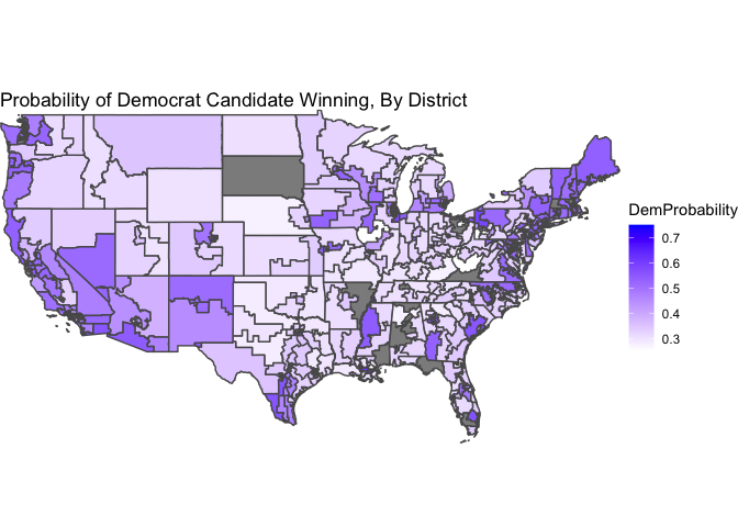
Below is a map of our district-level probabalistic predictions, where a color closer to white represents the Democrat winning with low probability, and a color closer to blue represents the Democrat winning with high probability. For clarity of the color scale, uncontested districts are not included in this map (because their probabilities are either 0 or 1).
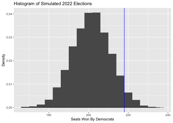
Finally, we can use this to form a final seat-share prediction. The sum of our Democrat win probabilities tells us the expected seat share for Democrats - the Democrats are predicted to win 202 seats, or 46.4%. We can also use simulation to show the distribution of Democrat seat wins, in the below histogram (where the vertical line denotes a majority).