Blog Post Three: Polls
September 19, 2022
The Economist’s and FiveThirtyEight’s Approaches
In this blog post, I will summarize the modeling approaches taken by two major political forecasters, The Economist and FiveThirtyEight. I will compare and contrast the two approaches, ultimately expressing a slight preference for FiveThirtyEight’s methodology, and will then update my predictive model using a couple of insights from both groups.
The Economist
In a nutshell, The Economist’s model approaches their prediction task in a two step process. The first step is to estimate the overarching national political sentiment - the nationwide popular vote shares that will be achieved by Democrats and Republicans. They use polling to inform this estimate. The primary source is the generic ballot poll, but they also consider polls of the president’s popularity (theorizing that a very popular president will tend to help their party’s congressional candidates, and vice versa). They adjust the estimates provided by the polls with such factors as the presence of uncontested seats, the degree of political polarization, and “fundamental” factors like the state of the economy and whether the election is a midterm.
In the second stage, The Economist uses this nationwide vote share forecast to individually predict each district. The idea is to use historical election data in that district to see how it tends to deviate from the national baseline. In addition to the raw historical vote shares, The Economist considers the presence of swing voters in the district, and structural factors like whether an incumbent is running, how much they’ve raised, and where they fall ideologically. Instead of making a point estimate from these factors, The Economist fits a skew-T distribution for each district, attempting to capture not just the most likely outcome but also the extreme events that might occur. With these distributions fitted, they make their final seat forecasts based on the proportion of seats won for each party in 10,000 simulations of the election.
FiveThirtyEight
This model predicts the midterm election in one step. The primary tool for this prediction is polling - and FiveThirtyEight uses pretty much any poll that they can get their hands on, as long as it comes from a professional source. Reflecting Galton’s observation that an aggregation of many guesses will tend to outperform one single guess, FiveThirtyEight takes great care to weight each poll appropriately. Weighting factors include how recently the poll was taken, the demographic of the poll (registered voters vs. likely voters), and the track record of the specific pollster. However, every single district will not have a poll dedicated to it, since only the most contested/followed/“interesting” ones will. So, FiveThirtyEight employs a k-nearest neighbors algorithm to predict what a hypothetical poll would say about an unpolled district, keeping in mind the selection bias of polls only being conducted in the more salient districts.
In addition to the polls, this model includes a diverse variety of fundamental variables that are known to impact the outcomes of elections. FiveThirtyEight includes on this list such factors as incumbency status, the margin of victory for the incumbent in the previous election, the generic ballot poll (as a measure of the national sentiment), campaign funds raised, the performance of the district in previous presidential and state legislative elections, and the political experience of the challenger. In races for open seats, only the relevant factors (so, those that do not relate to an incumbent) are included. One version of the FiveThirtyEight predictor even uses the ratings (“toss up”, “leans Democrat”, etc.) that historically accurate political experts have assigned each district. With all this in mind, FiveThirtyEight simulates many runs of the election, taking special care to model the correlation structure of the districts, to make its final prediction.
Comparing the Methods
The most obvious difference between the two methods is their overall structure. The Economist predicts a national trend and each district’s subsequent deviations from that trend, while FiveThirtyEight focuses exclusively on the idiosyncracies of each district. Within that structure, the models have many similarities in terms of the included variables. Both models include the fundamental factors that reflect the effect of structure on congressional elections - incumbency status, fundraising, whether it’s a midterm, and so on. The one notable difference in fundamentals is that The Economist includes the state of the economy (as indicated by the unemployment rate), while FiveThirtyEight does not include this (though, one might argue that it’s inclusion of Congress’s approval rating is relatively correlated to the state of the economy).
In terms of included variables, the major difference between the models lies not in the fundamentals but in the poll data. The Economist relies mostly on the generic ballot poll, while FiveThirtyEight uses a much wider variety of more specific polls (including the generic ballot poll in the fundamentals category as a representation of national sentiment). The reason for this difference is the reality that most individual districts will not have a poll targeted to it; the two forecasters just solve this problem with different methods. FiveThirtyEight applies k-nearest neighbors prediction to carefully-weighted averages of nearby polls, whereas The Economist instead ignores district-level polling and uses polls to predict a national baseline from which districts deviate in predictable ways.
Both forecasters take care to avoid giving too much weight to a single point estimate, but they again go about achieving this goal in different ways. The Economist uses elastic-net regularization to avoid large model coefficients that overfit the data, and then estimate a skew-T distribution (notorious for flexible shape and fat tails) for each district in order to adequately predict extreme events (making no mention of correlation between districts). FiveThirtyEight, on the other hand, makes no mention of regularization to scale down fitted coefficients, but they take great care to model the correlation structure between the error of each district’s estimate (taking into account four categories that describe how polls and fundamentals might over/understate certain factors across multiple districts). Both FiveThirtyEight and The Economist use simulation to reach their final predictions, most likely because the probability calculations required to find an analytic distribution would be intractable.
Both models obviously include a lot of thought, and were crafted by experienced data scientists. However, I believe FiveThirtyEight’s methodology to be slightly better, for two reasons. Firstly, while deviations from a national baseline is certainly a logical framework for this prediction task, it introduces two possible sources of error in the model: error in predicting the national vote share, and error in translating the national vote share to district vote shares. These errors might compound on each other in an “unlucky” realization of the election, so I marginally prefer FiveThirtyEight’s single-stage model, with only one prediction step in which an error could be made. Secondly, The Economist provided no justification for their assumption that each district follows a skew-T distribution, and it is well-known to be more difficult to learn an entire distribution than to learn a single parameter. So, while a fat-tailed and skewed distribution certainly makes sense, I again have a marginal preference for FiveThirtyEight’s approach of modeling the correlation structure between districts instead of the distributions of independent districts (especially considering the correlated polling errors we saw in 2016!). Again, though, I find both forecasts to be incredibly impressive.
2022 Forecast Update
In line with the FiveThirtyEight model, I update my model (that predicts vote share on a state-by-state level) to include the generic ballot poll. In accordance with the “wisdom of crowds” logic, I take a simple average of all generic ballot polls conducted within two months of the election - though, in the future, I would like to consider my weighting more carefully, as FiveThirtyEight does. For each poll average, I calculate the two-party vote share that would go to the Democrats. I also allow the presence of a Democrat in office to interact with the generic poll results, as voters might respond more favorably to Democrats if they are popular and a Republican president is in office.
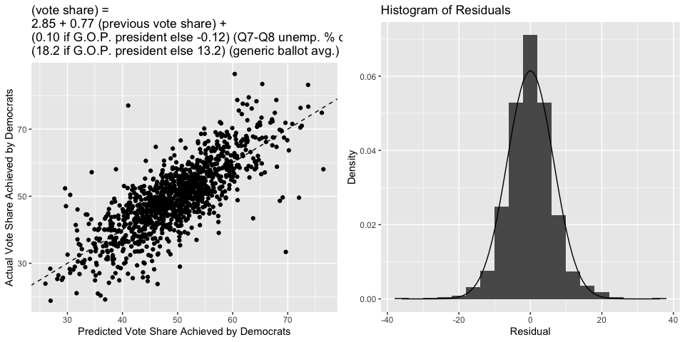
Interestingly, in this model, the economic variable that becomes more significant is the Q7-Q8 percent change in unemployment rate, not simply the Q8 unemployment rate. Last week, I concluded that voters tend to respond more to the absolute Q8 rate, so does this finding contradict that? It’s not quite that simple. Last week’s model isolated the effect of unemployment on voter choice, but this week’s model includes another variable (national sentiment via generic ballot) in the equation. So, an interpretation could be that once national sentiment is accounted for, voters respond more to the change in unemployment (perhaps because national sentiment is responsive to the overall level of unemployment).
Or, perhaps this just happened due to random chance. The coefficient on unemployment is significant, but still low - on the same order as it was last week. So, it might be the case that in this new model, since the effect of unemployment is relatively low in magnitude, the inclusion of a new covariate caused the percent change to become more significant due to pure chance. Indeed, the overall model is not very much improved from last week - the R-squared jumped by just around 1%, but the bootstrapped estimate of the root-mean squared decreases only to 6.51. In the future, the model might be improved by calibrating each state’s sensitivity to the national generic ballot poll separately (as, some states swing more than others), and by looking into district-level polls in addition to the generic ballot (as FiveThirtyEight does).
The two figures below include a scatterplot of the actual vote share to Democrats (each point is one state in one year) versus the predicted vote share. The fit looks pretty similar to last week’s fit (for reference, the dashed line indicates where the actual value would equal the predicted). On the right is a histogram of the residuals, with a Normal density overlayed. Again, the residuals appear normal, justifying our statistical inferences about this model.
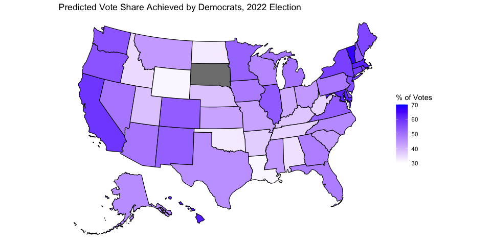
Below is a map that summarizes the point estimates of this model’s prediction of the 2022 election, using the most current available unemployment data and generic poll data. South Dakota again does not have a prediction because there is no Democrat running in the state. A color closer to blue corresponds to a larger vote share for Democrats, and a color closer to white corresponds to a smaller vote share for Democrats. Below is also a table that gives a 95% prediction interval for each state.
##             state LowerBound Predicted UpperBound
## 1         Alabama       21.1      33.9       46.7
## 2          Alaska       32.9      45.8       58.6
## 3         Arizona       36.3      49.1       61.9
## 4        Arkansas       23.9      36.7       49.5
## 5      California       46.3      59.3       72.3
## 6        Colorado       40.3      53.2       66.0
## 7     Connecticut       45.0      57.9       70.8
## 8        Delaware       42.2      55.0       67.7
## 9         Florida       35.4      48.2       61.0
## 10        Georgia       35.1      47.9       60.7
## 11         Hawaii       50.1      62.9       75.6
## 12          Idaho       22.0      34.9       47.7
## 13       Illinois       40.8      53.6       66.3
## 14        Indiana       28.6      41.3       54.1
## 15           Iowa       35.3      48.4       61.5
## 16         Kansas       29.8      42.6       55.4
## 17       Kentucky       24.8      37.6       50.4
## 18      Louisiana       18.4      31.2       44.0
## 19          Maine       43.4      56.4       69.5
## 20       Maryland       48.8      61.8       74.9
## 21  Massachusetts       49.1      62.0       75.0
## 22       Michigan       36.7      49.4       62.2
## 23      Minnesota       38.8      52.1       65.3
## 24    Mississippi       31.3      44.1       57.0
## 25       Missouri       29.6      42.6       55.5
## 26        Montana       31.2      43.9       56.7
## 27       Nebraska       25.4      38.2       51.0
## 28         Nevada       36.6      49.3       62.0
## 29  New Hampshire       40.5      53.6       66.7
## 30     New Jersey       42.9      55.8       68.7
## 31     New Mexico       39.9      52.7       65.5
## 32       New York       44.7      57.5       70.3
## 33 North Carolina       33.7      46.5       59.2
## 34   North Dakota       19.9      32.7       45.6
## 35           Ohio       31.2      44.0       56.8
## 36       Oklahoma       19.8      32.6       45.5
## 37         Oregon       41.7      54.5       67.3
## 38   Pennsylvania       35.8      48.6       61.4
## 39   Rhode Island       44.2      57.4       70.7
## 40 South Carolina       30.7      43.4       56.2
## 41      Tennessee       22.9      35.7       48.5
## 42          Texas       32.7      45.5       58.4
## 43           Utah       25.5      38.3       51.0
## 44        Vermont       53.7      66.8       79.8
## 45       Virginia       40.4      53.2       66.0
## 46     Washington       41.6      54.4       67.2
## 47  West Virginia       22.9      35.7       48.5
## 48      Wisconsin       34.0      46.8       59.5
## 49        Wyoming       18.3      31.2       44.0