Blog Post Eight: Final Midterm Prediction
November 7, 2022
Introduction
In this final blog post, I will present my final model for the 2022 midterm elections and its predictions for the composition of the House of Representatives.
Model Specification
Informed by all the work we have done over the past two months, our model will consist of two pieces.
The first piece will be an unpooled statewide model (so one model for each state) that predicts the Democrat’s vote share based on the economy, the generic ballot, the state’s previous vote share for Democrats, and structural election factors. We do not pool data across states because, as we saw last week, there is evidence of variation in the autocorrelation of different region’s vote shares. We go back to including the economy (as measured by the statewide unemployment rate) in this model because there is strong evidence for this variable’s impact in the literature, and it had legitimate predictive power our earlier state-level models.
The second piece will be a pooled district-level model that predicts the Democrat’s vote share based on expert ratings from Inside Elections and the Cook Political Report, demographic data, the incumbent’s ideological positioning as measured by DW-NOMINATE scores, and structural election factors. We pool this data because we expect these variables to affect all the districts similarly - for example, experts tune their ratings specifically to be consistent across districts, and there is strong evidence in the literature that the incumbent’s ideological positioning has a similar electoral effect across districts. Pooling also has the benefit of being more robust to redistricting, as we will end up with one model that applies to all districts, even those that were newly created after the 2020 census.
Finally, we will combine our two models via regression stacking, producing an ensemble model that will provide our final vote share prediction. We ultimately predict vote share, rather than seat share, to follow Jennifer Victor’s advice for effective presentation, and because in our previous work we did not see a large discrepancy in accuracy when predicting one versus the other.
Statewide Models
Formulation
Predictions of this model will follow the form
V̂i = logit(β0, i + (β1, iX1, i+β2, i)X2, i + β3, iX3, i + β4, iX4, i + β5, iX5, i)
Here, V̂i is the predicted vote share (for Democrats) in the ith state, each β is a coefficient, and each X is a variable. The subscript i on all the coefficients denote that this model allows each state to have its own coefficient. X1 is an indicator for whether the sitting president is a Democrat, X2 is the Q8 unemployment rate for the state, X3 is the results of the generic ballot poll (averaged over the month preceding the election), X4 is the state’s previous vote share for the Democrat candidate, and X5 is an indicator for whether the election is a midterm or not (where the sign indicates whether the sitting president is a Democrat or a Republican, since voters tend to punish the incumbent in midterms, not a particular party). This is essentially an unpooled version of our earliest model, with an added flag indicating whether it is a midterm year or a presidential year (which we saw proved useful in our most recent model).
Fit
We fit the models, and plot distributions of the coefficients to get a general sense of how predictions are made.
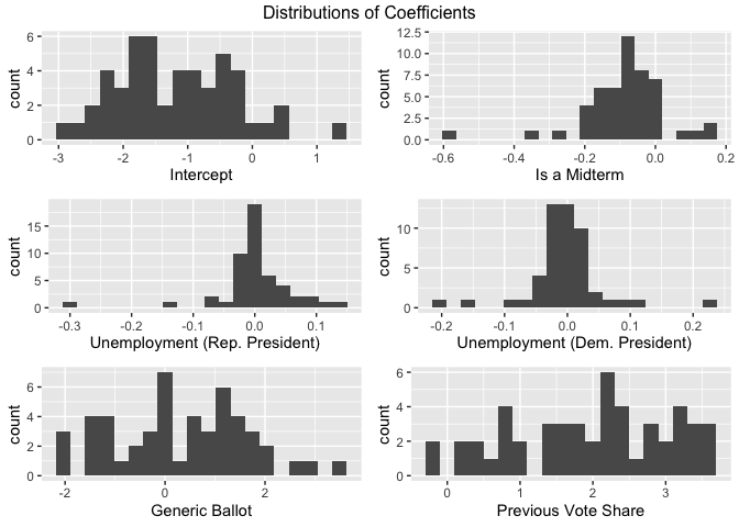
The magnitudes of the coefficients are difficult to interpret, since the variables all have different units and predictions are made via a logit function rather than a simple linear function. However, we can easily interpret the sign of the coefficients. Almost all of the models have a negative coefficient for the midterm flag, indicating that Democrats tend to receive fewer votes when it is a midterm and they have the presidency (and more votes when it is a midterm and a Republican has the presidency). Most of the models have a positive coefficient for the unemployment term when a Republican has the presidency, showing that voters turn to Democrats in periods of high unemployment because this is an issue they “own.” However, when a Democrat has the presidency, most of the coefficients shift to the left, showing that voters are less apt to “reward” Democrats for high unemployment when one is already president. There is a clean divide in the signs of the sensitivities to the generic ballot, indicating that some states are more conservative than the average voter and some states are more liberal than the average voter. Finally, almost all the models have positive sensitivity to their previous vote share, with some states being very sensitive to it and others being less so. For almost every model, all of the coefficients are statistically different from zero at a five percent significance level, which justifies this model.
District-Level Model
Formulation
Predictions of this model will follow the form
V̂i = logit(β0 + β1X1, i + β2X2, i + β3X3, i + β4X4, i + β5X5, i + β6X6, i + β7X7, i)
Here, V̂i is again the predicted vote share (for Democrats) in the ith district, each β is a coefficient, and each X is a variable. Notice that this time, the coefficients do not have a subscript i, so all districts share the same coefficients. X1 is the average rating from Inside Elections and the Cook Political Report (coded on a numerical scale), X2 is the proportion of the district below the age of 30, X3 is the proportion of the district that is female, X4 is the proportion of the district that is black or hispanic, X5 is the incumbent’s DW-NOMINATE score (the first dimension), X6 is a flag for the incumbency status of the seat (where the sign codes for Democrat versus Republican), and X7 is the same flag from the earlier model detailing the midterm status of the election and the party of the president.
Fit
We fit the models, and report the coefficients along with standard errors and p-values.
##
## Call:
## glm(formula = cbind(DemVotes, RepVotes) ~ Experts + `20_29` +
##     female + black_or_latino + nominate_dim1 + Incumbent + MidtermFlag,
##     family = binomial, data = pooled_df)
##
## Deviance Residuals:
##      Min        1Q    Median        3Q       Max
## -265.955   -51.968     1.303    47.671   299.987
##
## Coefficients:
##                   Estimate Std. Error z value Pr(>|z|)
## (Intercept)     -4.310e+00  5.110e-03 -843.50   <2e-16 ***
## Experts          1.036e-01  9.152e-05 1132.41   <2e-16 ***
## `20_29`          1.727e+00  3.729e-03  463.20   <2e-16 ***
## female           7.669e+00  9.545e-03  803.43   <2e-16 ***
## black_or_latino  4.281e-01  6.433e-04  665.54   <2e-16 ***
## nominate_dim1   -4.073e-01  5.231e-04 -778.55   <2e-16 ***
## Incumbent       -5.781e-03  2.551e-04  -22.66   <2e-16 ***
## MidtermFlag     -7.459e-02  1.654e-04 -451.06   <2e-16 ***
## ---
## Signif. codes:  0 '***' 0.001 '**' 0.01 '*' 0.05 '.' 0.1 ' ' 1
##
## (Dispersion parameter for binomial family taken to be 1)
##
##     Null deviance: 59701388  on 1869  degrees of freedom
## Residual deviance: 10676285  on 1862  degrees of freedom
## AIC: 10700241
##
## Number of Fisher Scoring iterations: 4
Again, we can much more easily interpret the signs of the coefficients than their magnitudes. The ratings of experts has a positive coefficient, which means that a district tends to see more votes for the Democrat when experts give it a stronger rating in favor of the Democrat. Each of the demographic categories we included has a positive sign, validating that (as we might have expected) these demographics tend to turn out more for Democrats than for Republicans. Between the categories, we actually can interpret the signs of the coefficients, because those three variables are all on the same scale - so we see that the Democrat’s vote share is most sensitive to the proportion of female voters, followed by the proportion of young voters, followed by the proportion of black and hispanic voters. The incumbent’s NOMINATE score has a negative coefficient, meaning that the Democrat gets more votes when the incumbent is more liberal and fewer votes when the incumbent is more conservative. The coefficient for the party of the incumbent is negative (but much smaller than the other coefficients), meaning that the Democrat gets slightly fewer votes when the incumbent is a Democrat and slightly more votes when the incumbent is a Republican. This is initially puzzling, but it seems that this coefficient is really measuring “regression to the mean,” as variables like the expert ratings and the incumbent’s NOMINATE score already implicitly account for the incumbency advantage. Finally, we again see that Democrats tend to receive fewer votes when it is a midterm and they have the presidency (and more votes when it is a midterm and a Republican has the presidency). All the coefficients are statistically significant, providing one justification for this model.
Final Ensemble Model and 2022 Prediction
Formulation
With the two component models in place, we are ready to specify how our final predictions will be made. The final prediction will take the form
V̂ = α0 + αunpooledSUMstates i(pi V̂unpooled, i) + αpooledMEANdistricts i(V̂pooled, i)
Again, the V̂’s represent predicted vote shares for the Democrats, with the left-hand side being a nationwide vote share prediction. The α’s represent the ensembling weights, where the pooled model gets one weight and the unpooled model gets another weight. To calculate the nationwide prediction of the unpooled model, we calculate the average prediction across all states, weighted by the state population p (according to the 2020 census). To calculate the nationwide prediction of the pooled model, we calculate the (unweighted) average prediction across all districts, which is reasonable because all districts have similar populations. This method of calculating a final prediction assumes that, across different states and districts, the proportion of eligible voters who turn out to vote is roughly the same. This is likely not an exact reflection of reality, but it should be close enough that a more nuanced calculation would make our model unnecessarily complicated.
Fit
To fit the α’s, we treat them as coefficients that we would like to learn via OLS (this is called “regression stacking”).
The fitted values are α0 = 0.09, αunpooled = − 0.3, and αpooled = 1.1. This is saying that the district-level model has a prediction that fluctuates more than the state-level models (which makes sense since the former is more granular than the latter). So, we “overpredict” with the district-level model, and then walk that prediction back using the state-level models.
Diagnostics
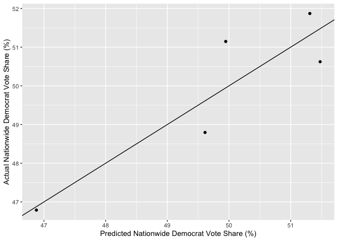
This model has an R-squared of 81%, meaning that we are able to explain 81% of the variation in the nationwide vote share attained by Democrats using this model. This is higher than any R-squared we had been able to achieve previously, which is exciting!
Here is a plot comparing the actual Democrat vote share to the predicted Democrat vote share in the five elections from the past decade (2012, 2014, 2016, 2018, and 2020), along with the 45-degree line for reference. All of the data points are very close to the line - within a vertical distance of 1 percentage point of the vote.
Using “leave one out” cross-validation, we can compute an out-of-sample estimate of the mean absolute prediction error. We find a mean absolute error of roughly 0.01, which means that our model will, on average, deviate from the true two-party vote share won by Democrats by around one percentage points. Expressed in terms of squared error instead of absolute error, the out-of-sample estimate for root-mean squared error is roughly two percentage points. Those are sizable margins, but they are lower than the other out-of-sample margins of error we encountered in our earlier work, which is also exciting!
2022 Prediction
After all this, we can make our final prediction for the 2022 midterm election. As always, we predict using the most current available values for all the predictors. Our point estimate is for Democrats to win 49.18% of the nationwide two-party vote share. To form a 95% prediction interval around this prediction, we calculate the standard error for each model and then apply the ensemble weights. The resulting prediction interval has Democrats winning between 49.15% and 49.21% of the nationwide two-party vote share. This is a very narrow predictive interval, and does not reflect the out-of-sample mean absolute error that we observed earlier. The problem here is described by FiveThirtyEight - we calculate standard errors as if the districts/states are independent of each other, but this is a very bad approximation of reality. In real life, the errors are quite correlated, which results in a much larger standard error than our calculation implies. This does not change the point estimate of our model, but it is a limitation that we must keep in mind when we interpret our accuracy post-election!
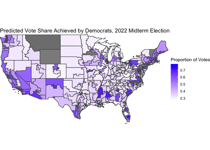
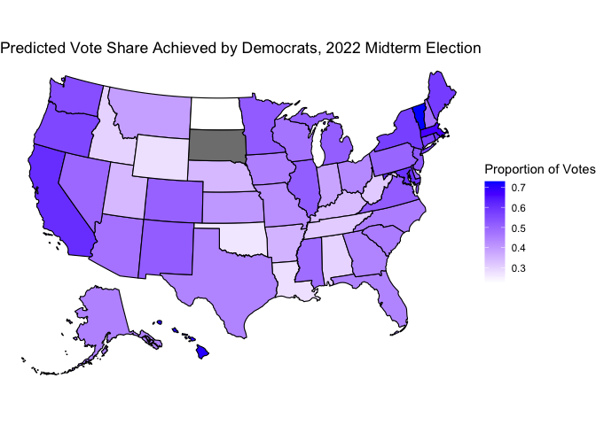
In an “appendix” section below, I include maps that visualize the individual predictions of the two models.
Below is a map of the statewide predictions (from the unpooled models). South Dakota has an uncontested election, so we do not include it on this map because our model does not apply to uncontested elections.
Below is a map of the district predictions (from the pooled model). The few grey districts (around 5) had data missing, so we do not include them on this map for simplicity.